In order to create spreadsheets in Excel it helps to know a few basic functions. These include merging cells, inserting data, formatting columns and rows and using borders and shading to easily identify groups of data.

To begin with, it helps to understand a bit of Excel jargon. The top row of menus are referred to as tabs (Home, Insert, Page Layout, etc.). This post will only be using the Home tab.

The menu that appears beneath the tab is called ‘the ribbon’. The ribbon contains the buttons you use to execute tasks (like Merge Cells).

Creating a heading by merging cells

To create a heading that runs over the top of a whole table:

1. Decide how wide the table will be roughly, you can always change it later.

2. Select the cells in the top row (rows go sideways, columns go up and down).

3. Hit the Merge & Center button.

To get a student list from eWorkSpace into your spreadsheet

1. Open eWorkSpace in Internet Explorer

2. Select Student Management on the left-hand side of the home screen.

3. Select Student Attendance Lists on the left-hand side of the Student Management page.

4. Select the class. Your list will appear below.

5. Highlight the students’ names in the list and copy (Ctrl+C)

6. Open the spreadsheet and select the first cell under your heading (probably A2) and paste (Ctrl+V)

Resizing the cells

By now your students’ names will be hanging over the edges of their boxes so we need to resize the A column. To do so, put the cursor between the A and the B column at the top and double-click. This should automatically resize column A to the width of the longest student’s name.

If you want to resize a range of cells to a particular size manually, select the range of columns or cells at the edge of the table (see diagram below), right-click and select resize column/row. This will open up a dialogue box where you can enter the width of you require (say 10 or 20, just play around with it).

Adding a row or column

If you want to enter a new student or a second tier of headings, insert a new row or column by right-clicking the letter or number at the edge of the table (see above) and selecting Insert. This will put a new row above the row you click on or before the column you select.

Adding a border

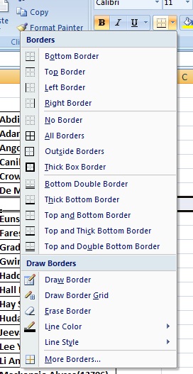
Excel spreadsheets look like they have a border around them already so you might be surprised, when you go to print them, that they actually don’t. To put one in, select the area you want the borders to be around from top-right to bottom-left then click the arrow next to the Border button on the Home tab (pictured below). This will open a drop down menu where you can choose how many sides your border has. Select All borders.

The borders will appear (and print out) the range that you select so if you go beyond the limits of your data, you will get a print out of heaps of pages of empty cells.

Adding Shading

You might also like to make your data more readable by adding shading. To do this, follow the steps below:

1. Select the range of data you want to format. Since you probably don’t want to include the heading row, start from the first row that contains data.

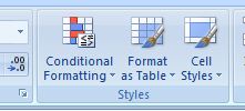
2. Click the Conditional Formatting button (pictured below).

3. This will open a menu. Select ‘New Rule…’

4. From the six options that appear in the dialogue box that this has opened, click the last one, ‘Use a formula to detemine which cells to format’.

5. This will change the bottom of this dialogue box so that a field appears labelled ‘Format values where this formula is true:’. Into this cell, copy and paste the following formula: =MOD(ROW(),2)=0

6. Below this field, click the Format button. By selecting the Fill tab in the dialogue box that opens, you can choose the colour that will be applied to every other row.

7. Select the colour then click ok on all the dialogue boxes that are open to make them go away and to apply your zippy shading.

Changing the text direction

Excel has a button just for this. It looks like this:

Clicking this button will open up a drop-down menu where you can specify whether you want the text to appear: on an angle, coming from the top going down, bottom up, etc.