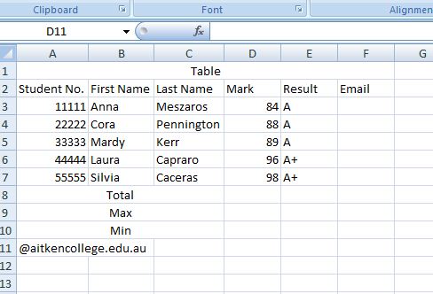
Excel has a range of functions that can be used in your spreadsheet to manipulate your data. Some of the simple things you might like to do are to work out the sum of a column, the highest and lowest numbers in that column and to merge two cells together. In order to do this, I will be using the table below.

Showing leading zeros

As you can see from the table above, I have been tricky and avoided the whole leading zero issue by using student numbers without them. You will probably have some students in your class who have a zero or zeros at the front of their student number and, for various reasons, you want to see them. Here’s how it’s done:

1. Select the cell range (in this case A3:A7).

2. Click on the button in the bottom right-hand corner of the numbers bit of the ribbon (pictured below).

3. This will open a dialogue box and should already be in the numbers menu. Select Custom and in the field under the word ‘Type:’ enter five zeros.

This will tell Excel that these cells should have a five digit number in them irrespective of zeros at the beginning.

Sorting the data A-Z

The first thing that I want to do is to put my students into alphabetical order but Excel wants to have them sorted by Student no. (actually, Excel is a computer program so who knows what it wants). In order to sort them by last name I…

1. Select from cell A2 down to F7.

2. Right-click the data that I have selected.

3. Select Sort> Custom Sort

4. In the ‘Sort by” drop-down menu in the dialogue box that appears (that Excel has cleverly filled with the information that you have put in the second row), select ‘Last Name’.

5. Click ok and your table should be organised alphabetically by last name.

Getting a total

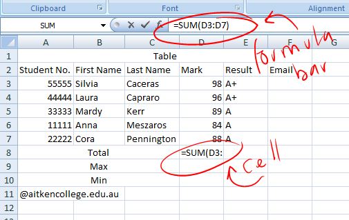
This is not a spectacular example of a table that you would want a total figure for but the principle is the same for all equations. To get a total of the marks column, do the following:

1. Select the cell where you want to total to appear, in this case D8.

2. In the formula bar or the cell itself (pictured above), type =SUM(

3. Using the mouse pointer, select the range you want to add up by clicking the first cell in the range and dragging down to the last cell. This should then flash blue.

4. While it is flashing hit enter. This will complete the equation and the total should appear in the designated cell.

Alternatively, you can type the whole equation in the desired cell like this: =SUM(D3:D7)

Other equations

Follow the same process for the following equations using the formulas below:

Minimum occurring number: =MIN(Cell range)

Maximum occurring number: =MAX(Cell range)

Average of a column: =AVERAGE(Cell range)

So what’s with the cell that says “@aitkencollege.edu.au”?

That was a mistake. But it was there to illustrate that there is this really handy function called concatenate. Cancatenate will merge the data in two cells into a third cell. This is handy if you have the students first name in one column and their second name in the second. You can concatenate these two columns of data into one column that includes both bits of information. Extremely handy when you are setting up job lots of student accounts and you want to use their user number and first name for their username. Here’s how:

1. In a cell next to your table (in the example above that would be F3) create the formula: =CONCATENATE(A3, B3)

2. Fill down by holding the mouse pointer over the bottom, right-hand corner of the cell (the fat white cross will turn into a thin black cross), click and drag to the bottom of your table. This will automatically put in the formula for the rest of the cells.

Separating two field with a comma will put them next to each other without a space. If you want a space, use this format (A3, ” “, B3).

If you want to create an email list, write the formula like this and then fill down: =CONCATENATE(A3, “@aitkencollege.edu.au”)